NEPAL is to calculate neuroendocrine (NE) risk score from bulk and single-cell transcriptomics of both human and mouse prostate cancer (PCa). NEPAL has multiple built-in algorithms and NE gene sets. NEPC risk score may be used to stratify prognosis of PCa.
Graphical Abstract:
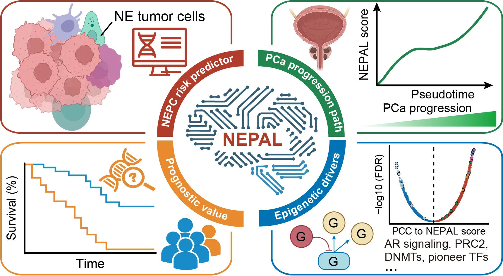
Integrated analysis of single-cell and bulk transcriptomics develops a robust neuroendocrine cell-intrinsic signature to predict prostate cancer progression
Tingting Zhang#, Faming Zhao#※, Yahang Lin, Mingsheng Liu, Hongqing Zhou, Fengzhen Cui, Yang Jin, Liang Chen, Xia Sheng※
Zhang T, Zhao F, Lin Y, Liu M, Zhou H, Cui F, Jin Y, Chen L, Sheng X. Integrated analysis of single-cell and bulk transcriptomics develops a robust neuroendocrine cell-intrinsic signature to predict prostate cancer progression. Theranostics 2024; 14(3):1065-1080. doi:10.7150/thno.92336. https://www.thno.org/v14p1065.htm
PMID: 38250042 DOI: 10.7150/thno.92336
Xia Sheng, PhD, xiasheng@hust.edu.cn
Key Laboratory of Environmental Health, Ministry of Education & Ministry of Environmental Protection, School of Public Health, Tongji Medical College, Huazhong University of Science and Technology, Wuhan, China.
Any technical question please contact Faming Zhao (famingzhao@hust.edu.cn) or Tingting Zhang (tingtingzhang@hust.edu.cn).
copyright, ShengLab@HUST
You may install this package with:
# options("repos"= c(CRAN="https://mirrors.tuna.tsinghua.edu.cn/CRAN/"))
# options(BioC_mirror="http://mirrors.tuna.tsinghua.edu.cn/bioconductor/")
if (!requireNamespace("BiocManager", quietly = TRUE)) install.packages("BiocManager")

#IOBR is an R package to perform comprehensive analysis of tumor microenvironment and signatures for immuno-oncology.
# devtools::install_github("IOBR/IOBR")

list.of.packages <- c("dplyr", "survival", "survminer", "ggplot2", "biomaRt",
                      "e1071","GSVA","glmnet","devtools", "Seurat","AUCell")
#checking missing packages from list
new.packages <- list.of.packages[!(list.of.packages %in% installed.packages()[,"Package"])]
packToInst <- setdiff(list.of.packages, installed.packages())

lapply(packToInst, function(x){
  BiocManager::install(x,ask = F,update = F)
})

# You can install NEPAL from Github:
devtools::install_github("Famingzhao/NEPAL")
## load R package and internal data set
library(NEPAL)
load(system.file("data", "demo.Bulk.RData", package = "NEPAL", mustWork = TRUE)) # load example data

## calculate NE scores using NEPAL gene sets and ssGSEA method
NE.scores.ssgsea = NEPAL_bulk(bulk.data = WCDT_expr,
                                    method = "ssGSEA", #method = c("ssGSEA","Enet","Ridge","SVM","all")
                                    species="human", #species=c("human","mouse")
                                    gene.sets="NEPAL")
# gene.sets = c("all","EurUrol.2005", "CancerDiscov.2011", "CancerRes.2014", "NatMed.2016",
#               "CellRep.2018.scRNA", "ClinCancerRes.2015", "JClinInvest.2019",
#               "IntJCancer.2019", "HP_NE_neoplasm", "JClinOncol.2018", "BMC.Cancer.2017","NEPAL")

## print
head(NE.scores.ssgsea)
# ID Index   NE_sig_UP NE_sig_DN   NE_UP_DN
# 1 DTB-003     1  0.47120891 0.2867273  0.1844816
# 2 DTB-005     2 -0.07352663 0.6371859 -0.7107125
# 3 DTB-008     3 -0.13467574 0.5162950 -0.6509708
# 4 DTB-009     4 -0.07574755 0.5896833 -0.6654309
# 5 DTB-011     5 -0.22116854 0.6971295 -0.9182981
# 6 DTB-018     6 -0.11747824 0.7080533 -0.8255315

## or users also can calculate NE scores using machine learning algorithms
NE.scores.all = NEPAL_bulk(bulk.data = WCDT_expr,
                                 method = c("all"),
                                 species="human")
## print
head(NE.scores.all)
# ID Index   NE_sig_UP NE_sig_DN   NE_UP_DN   alpha.0 alpha.0.1 alpha.0.2 alpha.0.3 alpha.0.4 alpha.0.5
# 1 DTB-003     1  0.47120891 0.2867273  0.1844816 0.9073267 0.8644939 0.8194201 0.8188917 0.8344952 0.8415515
# 2 DTB-005     2 -0.07352663 0.6371859 -0.7107125 0.3542819 0.3669717 0.4149525 0.4753370 0.4905505 0.5072813
# 3 DTB-008     3 -0.13467574 0.5162950 -0.6509708 0.3290364 0.3427523 0.4021970 0.4803067 0.5057132 0.5191514
# 4 DTB-009     4 -0.07574755 0.5896833 -0.6654309 0.4112042 0.4762680 0.4809674 0.5129319 0.5335130 0.5504454
# 5 DTB-011     5 -0.22116854 0.6971295 -0.9182981 0.3296918 0.3780843 0.4121598 0.4413186 0.4431671 0.4439999
# 6 DTB-018     6 -0.11747824 0.7080533 -0.8255315 0.3206407 0.3597761 0.3816835 0.4119724 0.4191327 0.4204871
# alpha.0.6 alpha.0.7 alpha.0.8 alpha.0.9   alpha.1 Ridge.score SVM.score
# 1 0.8478319 0.8428098 0.8360111 0.8305164 0.8212084   0.9999918 0.8237709
# 2 0.5148875 0.5319407 0.5354641 0.5389421 0.5400744   0.9787062 0.3630503
# 3 0.5288195 0.5368882 0.5419930 0.5479270 0.5505872   0.9701211 0.2257297
# 4 0.5624224 0.5814033 0.5926642 0.6039962 0.6109182   0.9901306 0.6156952
# 5 0.4388316 0.4493126 0.4534616 0.4584895 0.4598450   0.9703820 0.1705570
# 6 0.4139546 0.4320603 0.4331922 0.4342733 0.4304872   0.9665735 0.3707302
library(survminer)
library(survival)
library(ggplot2)

table(row.names(WCDT_phe) == NE.scores.ssgsea$ID)
# TRUE
# 66
WCDT_phe = cbind(WCDT_phe,NE.scores.ssgsea[,-c(1,2)])

WCDT_phe$OS.mCRPC # days
WCDT_phe$OS.month = WCDT_phe$OS.mCRPC/30

# find optimal cutoff by Survminer or customized definition by user
cut <- surv_cutpoint(WCDT_phe,
                     'OS.month','Event','NE_UP_DN')
print(paste0('The optimal cutpoint is ',cut$cutpoint$cutpoint,'.'))

WCDT_phe$NE_group = ifelse(WCDT_phe$NE_UP_DN> cut$cutpoint$cutpoint,
                           "High","Low") %>% factor(levels = c("Low","High"))

WCDT_fit_os <- survfit(Surv(OS.month, Event)~NE_group,
                        data= WCDT_phe)
ggsurvplot(WCDT_fit_os, conf.int=F, pval=TRUE,risk.table = F)

# Vis using `draw.survival` built-in function
draw.survival(survfit= WCDT_fit_os,ylab= "OS",
              legend.position = "top",
              plot.title ="WCDT CRPC/Met",
              break.time = NA, xlimt = NA,
              palette = c('NE.sig Low' = "#1F78B4",
                          'NE.sig High'="#E31A1C"),
              legend.labs = c('NE.sig Low','NE.sig High'),
             risk.table = F,front.size = 12)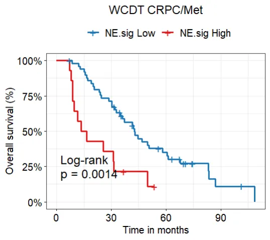
## load internal GSE69903 mouse data set
load(system.file("data","demo.Mus.Bulk.RData",package = "NEPAL", mustWork = TRUE)) # load example data

## calculate NE scores using NEPAL gene sets and ssGSEA method
NE.mus.ssgsea = NEPAL_bulk(bulk.data = GSE69903_mus_expr,
                                    method = "ssGSEA", #method = c("ssGSEA","Enet","Ridge","SVM","all")
                                    species = "mouse", #species=c("human","mouse")
                                    gene.sets = "NEPAL")
head(NE.mus.ssgsea)
table(row.names(GSE69903_mus_phe) == NE.mus.ssgsea$ID)
# TRUE
# 29
GSE69903_mus_phe = cbind(GSE69903_mus_phe,NE.mus.ssgsea[,-c(1,2)])

## Vis
if(T){
  mytheme <- theme(plot.title = element_text(size = 10,color="black",hjust = 0.5),
                   axis.ticks = element_line(color = "black"),
                   axis.title = element_text(size = 8,color ="black"),
                   axis.text = element_text(size = 8,color = "black"),
                   axis.text.x = element_text(angle = 90, hjust = 0.5),
                   panel.grid=element_blank(),
                   legend.position = "right",
                   legend.text = element_text(size = 8),
                   legend.title= element_text(size = 8),
                   panel.border = element_rect(fill = NA,color = "black", size = 0.8, linetype = "solid"),
                   strip.background = element_rect(color ="black",size = 1, linetype ="solid")
  )
}

GSE69903_mus_phe$Group
GSE69903_mus_phe$Group = factor(GSE69903_mus_phe$Group,
                                levels = c("Non-NE","NEPC"))

GSE69903_mus_phe = GSE69903_mus_phe[order(GSE69903_mus_phe$NE_UP_DN),]
GSE69903_mus_phe$geo_accession = factor(GSE69903_mus_phe$geo_accession,
                                        levels = GSE69903_mus_phe$geo_accession)

p.mus = ggplot(GSE69903_mus_phe,
               mapping = aes(x = geo_accession,y= NE_UP_DN,fill=Group))+
    geom_bar(stat = "identity",width = 1,color="black") +
    # coord_cartesian(expand = 0,clip = 'off') +
    # scale_y_continuous(limits = c(-1,0.25))+
    theme_bw()+ theme(axis.text.x = element_text(angle = 90,vjust = 0.5))+
    labs(x=NULL,y="NE_UP_DN (ssGSEA)",title = "GSE69903 mouse (n=29)")+
    scale_fill_manual(values = c("Non-NE" = "#0072B5FF","NEPC" = "#BC3C29FF"))+mytheme
p.mus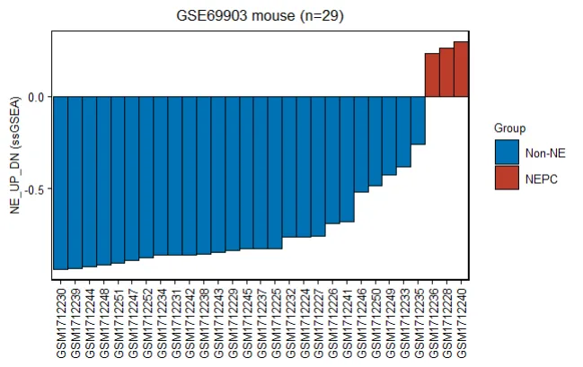
## load R package and internal data set
library(NEPAL)
library(Seurat)
seurat.data = readRDS(system.file("data", "NatMed.He.2021.Rds",
package = "NEPAL", mustWork = TRUE))
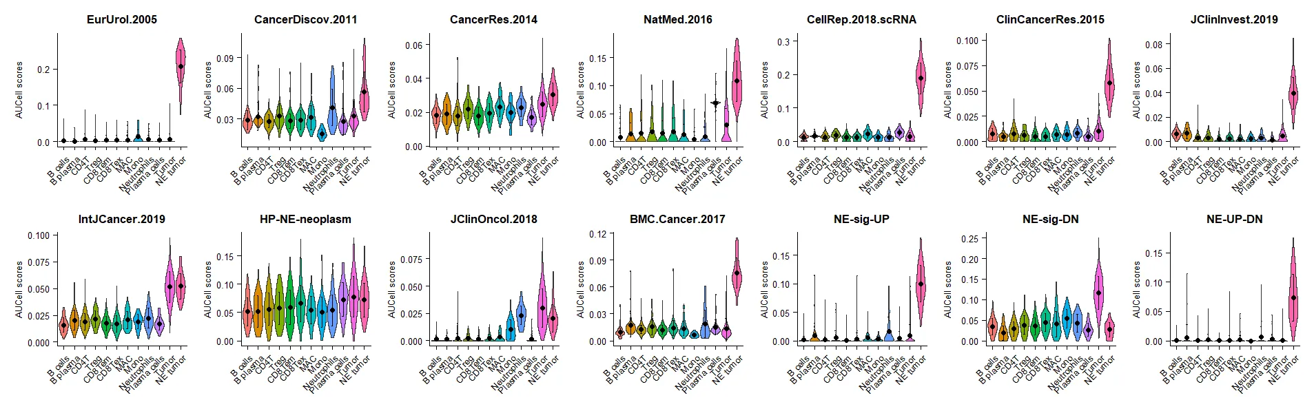
## calculate NE scores using NEPAL and published gene sets based on AUCell method
NE.seurat = NEPAL_scRNA(seurat.data=seurat.data,
method = "AUCell",
species= "human",
ncores=1,
assay.names = "NE",
DefaultAssay=F)
NE.seurat
# An object of class Seurat
# 25492 features across 1954 samples within 2 assays
# Active assay: RNA (25478 features, 0 variable features)
# 1 other assay present: NE
## print
NE.seurat@assays$NE@data[1:10,1:5]
# 0 1 2 3 4
# EurUrol.2005 . . . . .
# CancerDiscov.2011 0.030069409 0.028371479 0.027095164 0.05537486 0.0309613951
# CancerRes.2014 0.028906723 0.027093847 0.030111064 0.03363752 0.0307297846
# NatMed.2016 . . . 0.05425526 .
# CellRep.2018.scRNA 0.015979749 . . 0.02746803 0.0159667684
# ClinCancerRes.2015 0.014439507 . 0.023929059 0.01329820 0.0058283802
# JClinInvest.2019 0.004972814 0.003544499 0.002545555 . 0.0004600400
# IntJCancer.2019 0.045452989 0.020250315 0.037110596 0.04981038 0.0257334372
# HP-NE-neoplasm 0.171063411 0.048336883 0.106668851 0.04021441 0.0676716369
# JClinOncol.2018 0.027398209 . 0.039934695 0.03074259 .
# BMC.Cancer.2017 0.015587477 0.018236955 0.003543278 0.02679190 0.0201031308
# NE-sig-UP 0.001904375 0.010594900 0.002146047 0.03352474 0.0001256694
# NE-sig-DN 0.153510172 0.013322696 0.128280814 0.04104507 0.0314120463
# NE-UP-DN . . . . .
## Vis
p2 = VlnPlot(NE.seurat,
pt.size = 0,
group.by = "celltype",
features = row.names(NE.seurat@assays$NE@data),
assay = "NE",
stack = F,ncol = 7)&
labs(x=NULL,y="AUCell scores")&
stat_summary(fun = "mean", geom = "point",position = position_dodge(0.9)) &
stat_summary(fun.data = "mean_sd", geom = "errorbar", width = .15,
size = 0.3,position = position_dodge(0.9))&
theme(plot.title = element_text(size = 10,color="black",hjust = 0.5),
axis.ticks = element_line(color = "black"),
axis.title = element_text(size = 8,color ="black"),
axis.text = element_text(size=8,color = "black"),
axis.text.x = element_text(angle = 45, hjust = 1 ),
panel.grid=element_blank(),
legend.position = "none",
legend.text = element_text(size= 8),
legend.title= element_text(size= 8),
strip.background = element_rect(color="black",size= 1, linetype="solid") # fill="#FC4E07",
);p2