Poly2Graph

Poly2Graph is a Python package for automatic Hamiltonian spectral graph construction. It takes in the characteristic polynomial and returns the spectral graph.

Topological physics is one of the most dynamic and rapidly advancing fields in modern physics. Conventionally, topological classification focuses on eigenstate windings, a concept central to Hermitian topological lattices (e.g., topological insulators). Beyond such notion of topology, we unravel a distinct and diverse graph topology emerging in 1D crystal's energy spectra (under open boundary condition). Particularly, for non-Hermitian crystals, their spectral graphs features a kaleidoscope of exotic shapes like stars, kites, insects, and braids.

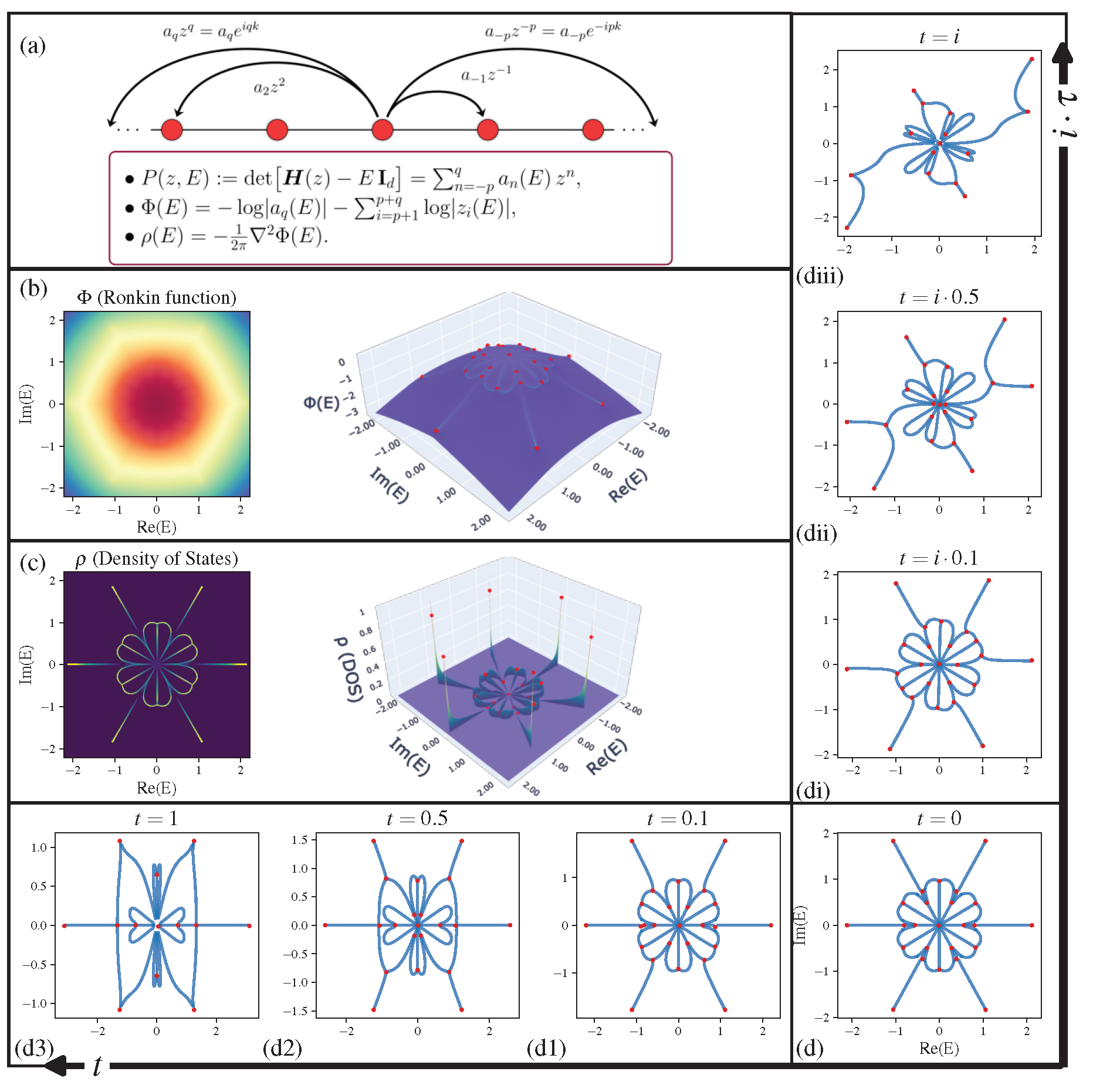
Figure: Poly2Graph Pipeline — (a) Starting from a 1-D crystal Hamiltonian $H(z)$ in momentum space — or, equivalently, its characteristic polynomial $P(z,E)=\det[\mathbf{H}(z)-E\mathbf{I}]$. The crystal’s open-boundary spectrum solely depends on $P(z,E)$. (b) The spectral potential $\Phi(E)$ (Ronkin function) is computed from the roots of $P(z,E)=0$, following recent advances in non-Bloch band theory. (c) The density of states $\rho(E)$ is obtained as the Laplacian of $\Phi(E)$. (d) The spectral graph is extracted from $\rho(E)$ via a morphological computer-vision pipeline. Varying the coefficients of $P(z,E)$ produces diverse graph morphologies in the real domain (d1)–(d3) and imaginary domain (di)–(diii).

Features

• Poly2Graph
  1. High-performance
     • Fast construction of spectral graph from any one-dimensional models
     • Adaptive resolution to reduce floating operation cost and memory usage
     • Automatic backend for computation bottleneck. If tensorflow / torch is available, any device (e.g. '/GPU:0', '/TPU:0', 'cuda:0', etc.) that they support can be used for acceleration.
  2. Cover generic topological lattices
     • Support generic one-band and multi-band models
     • Flexible multiple input choices, be they characteristic polynomials or Bloch Hamiltonians; formats include strings, sympy.Poly, and sympy.Matrix
  3. Automatic and Robust
     • By default, no hyper-parameters are needed. Just input the characteristic of your model and poly2graph handles the rest
     • Automatic spectral boundary inference
     • Relatively robust on multiband models that are prone to "component fragmentation"
  4. Helper functionalities generally useful
     • skeleton2graph module: Convert a skeleton image to its graph representation
     • hamiltonian module: Conversion among different Hamiltonian representations and efficient computation of a range of properties

Installation

You can install the package via pip:

$ pip install poly2graph

or clone the repository and install it manually:

$ git clone https://github.com/sarinstein-yan/poly2graph.git
$ cd poly2graph
$ pip install .

Optionally, if TensorFlow or PyTorch is available, poly2graph will make use of them automatically to accelerate the computation bottleneck. Priority: tensorflow > torch > numpy.

This module is tested on Python >= 3.11. Check the installation:

import poly2graph as p2g
print(p2g.__version__)

Usage

See the Poly2Graph Tutorial JupyterNotebook.

p2g.SpectralGraph and p2g.CharPolyClass are the two main classes in the package.

p2g.SpectralGraph investigates the spectral graph topology of a specific given characteristic polynomial or Bloch Hamiltonian. p2g.CharPolyClass investigates a class of parametrized characteristic polynomials or Bloch Hamiltonians, and is optimized for generating spectral properties in parallel.

import numpy as np
import networkx as nx
import sympy as sp
import matplotlib.pyplot as plt

# always start by initializing the symbols for k, z, and E
k = sp.symbols('k', real=True)
z, E = sp.symbols('z E', complex=True)

A generic one-band example (p2g.SpectralGraph):

characteristic polynomial:

$$P(E,z) := h(z) - E = z^4 -z -z^{-2} -E$$

Its Bloch Hamiltonian (Fourier transformed Hamiltonian in momentum space) is a scalar function:

$$h(z) = z^4 - z - z^{-2}$$

where the phase factor is defined as $z:=e^{ik}$.

Expressed in terms of crystal momentum $k$:

$$h(k) = e^{4ik} - e^{ik} - e^{-2ik}$$

---

The valid input formats to initialize a p2g.SpectralGraph object are:

1. Characteristic polynomial in terms of z and E:
   • as a string of the Poly in terms of z and E
   • as a sympy.Poly with {z, 1/z, E} as generators
2. Bloch Hamiltonian in terms of k or z
   • as a sympy.Matrix in terms of k
   • as a sympy.Matrix in terms of z

All the following characteristics are valid and will initialize to the same characteristic polynomial and therefore produce the same spectral graph:

char_poly_str = '-z**-2 - E - z + z**4'

char_poly_Poly = sp.Poly(
    -z**-2 - E - z + z**4,
    z, 1/z, E # generators are z, 1/z, E
)

phase_k = sp.exp(sp.I*k)
char_hamil_k = sp.Matrix([-phase_k**2 - phase_k + phase_k**4])

char_hamil_z = sp.Matrix([-z**-2 - E - z + z**4])

Let us just use the string to initialize and see a set of properties that are computed automatically:

sg = p2g.SpectralGraph(char_poly_str, k=k, z=z, E=E)

---

Characteristic polynomial:

sg.ChP

>>> $\text{Poly}{\left( z^{4} - z -\frac{1}{z^{2}} - E, ~ z, \frac{1}{z}, E, ~ domain=\mathbb{Z} \right)}$

---

Bloch Hamiltonian:

• For one-band model, it is a unique, rank-0 matrix (scalar)

sg.h_k

>>>

$$\begin{bmatrix}e^{4 i k} - e^{i k} - e^{- 2 i k}\end{bmatrix}$$

sg.h_z

>>>

$$\begin{bmatrix}- \frac{- z^{6} + z^{3} + 1}{z^{2}}\end{bmatrix}$$

---

The Frobenius companion matrix of P(E)(z):

• treating E as parameter and z as variable
• Its eigenvalues are the roots of the characteristic polynomial at a fixed complex energy E. Thus it is useful to calculate the GBZ (generalized Brillouin zone), the spectral potential (Ronkin function), etc.

sg.companion_E

>>>

$$\begin{bmatrix}0 & 0 & 0 & 0 & 0 & 1 \\ 1 & 0 & 0 & 0 & 0 & 0 \\ 0 & 1 & 0 & 0 & 0 & E \\ 0 & 0 & 1 & 0 & 0 & 1 \\ 0 & 0 & 0 & 1 & 0 & 0 \\ 0 & 0 & 0 & 0 & 1 & 0\end{bmatrix}$$

---

Number of bands & hopping range:

print('Number of bands:', sg.num_bands)
print('Max hopping length to the right:', sg.poly_p)
print('Max hopping length to the left:', sg.poly_q)

>>>

Number of bands: 1
Max hopping length to the right: 2
Max hopping length to the left: 4

---

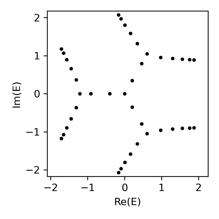
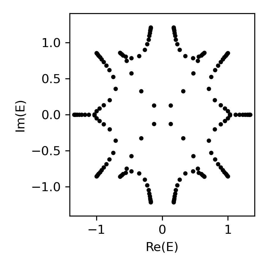
A real-space Hamiltonian of a finite chain and its energy spectrum:

H = sg.real_space_H(
    N=40,        # number of unit cells
    pbc=False,   # open boundary conditions
    max_dim=500  # maximum dimension of the Hamiltonian matrix (for numerical accuracy)
)

energy = np.linalg.eigvals(H)

fig, ax = plt.subplots(figsize=(3, 3))
ax.plot(energy.real, energy.imag, 'k.', markersize=5)
ax.set(xlabel='Re(E)', ylabel='Im(E)', \
xlim=sg.spectral_square[:2], ylim=sg.spectral_square[2:])
plt.tight_layout(); plt.show()

---

The Set of Spectral Functions

(whose values plotted on the complex energy square, returned as a 2D array)

• Density of States (DOS)

  Defined as the number of states per unit energy area in the complex energy plane.

  $$\rho(E) = \lim_{N\to\infty}\sum_n \frac{1}{N} \delta(E-\epsilon_n)$$

  where $\epsilon_n$ are the eigenvalues of the Hamiltonian $H$.

  Imagine to assign electric charge $1/N$ to each eigenvalue $\epsilon_n$, then the density of states $\rho(E)$ is treated as a charge density, therefore can be interpreted as the laplacian of a spectral potential $\Phi(E)$:

  $$\rho(E) = -\frac{1}{2\pi} \Delta \Phi(E)$$

  $\Delta = \partial_{\text{Re} E}^2 + \partial_{\text{Im} E}^2$ is the Laplacian operator on the complex energy plane. Laplacian operator extracts curvature; thus, geometrically speaking, the loci of spectral graph $\mathcal{G}$ resides on the ridges of the Coulomb potential landscape.

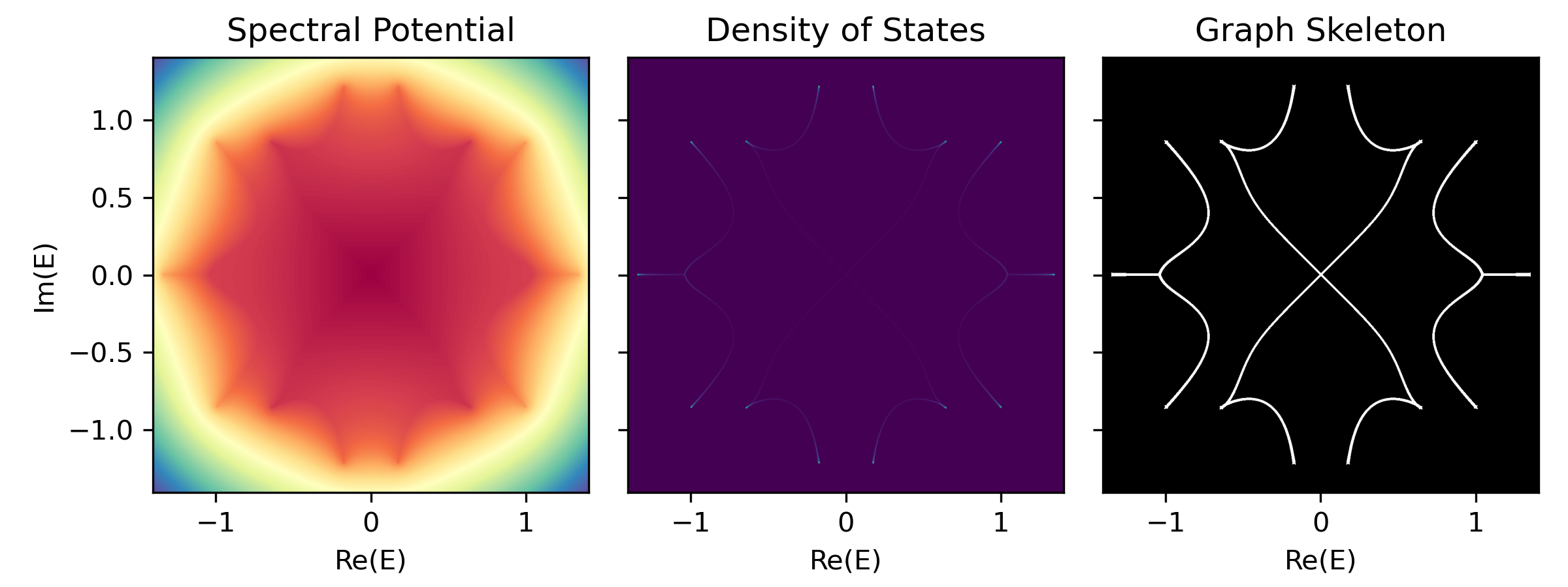
• Spectral Potential (Ronkin function)

  It can be proven that the spectral potential $\Phi(E)$ can be efficiently computed from the roots $|z_i(E)|$ of the characteristic polynomial $P(E)(z)$ and the leading coefficient $a_q(E)$ at a complex energy $E$:

  $$\Phi(E) = - \lim_{N\to\infty} \sum_{\epsilon_n} \log|E-\epsilon_n| \ = - \int \rho(E')\log|E-E'| d^2E' \ = - \log|a_q(E)| - \sum_{i=p+1}^{p+q} \log|z_i(E)|$$

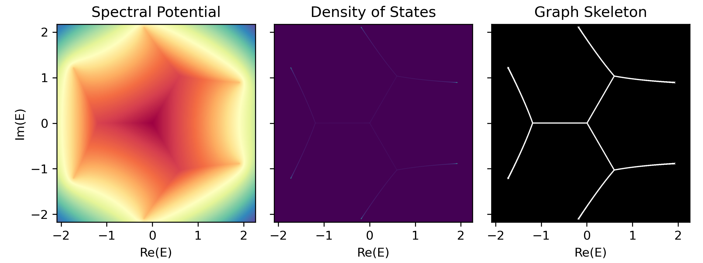
• Graph Skeleton (Binarized DOS)

phi, dos, binaried_dos = sg.spectral_images()

fig, axes = plt.subplots(1, 3, figsize=(8, 3), sharex=True, sharey=True)
axes[0].imshow(phi, extent=sg.spectral_square, cmap='terrain')
axes[0].set(xlabel='Re(E)', ylabel='Im(E)', title='Spectral Potential')
axes[1].imshow(dos, extent=sg.spectral_square, cmap='viridis')
axes[1].set(xlabel='Re(E)', title='Density of States')
axes[2].imshow(binaried_dos, extent=sg.spectral_square, cmap='gray')
axes[2].set(xlabel='Re(E)', title='Graph Skeleton')
plt.tight_layout()
plt.show()

---

The spectral graph $\mathcal{G}$

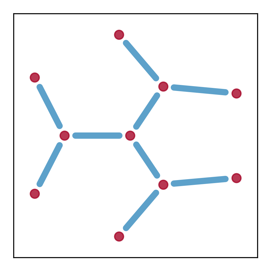
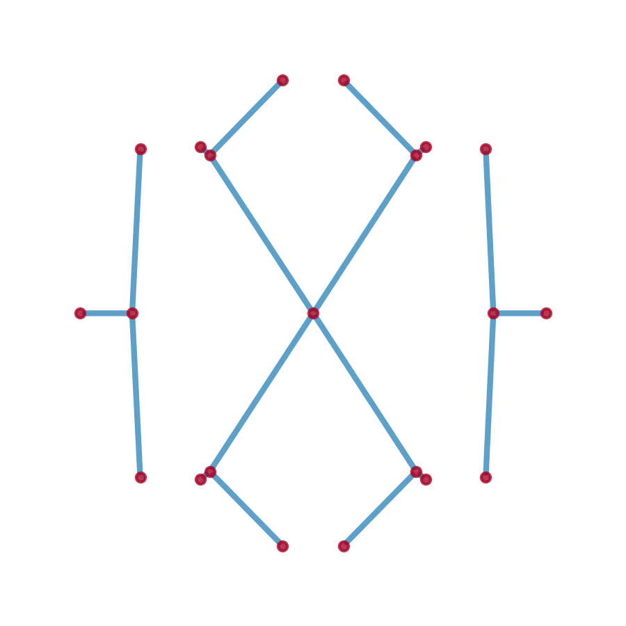
graph = sg.spectral_graph()

fig, ax = plt.subplots(figsize=(3, 3))
pos = nx.get_node_attributes(graph, 'pos')
nx.draw_networkx_nodes(graph, pos, alpha=0.8, ax=ax,
            node_size=50, node_color='#A60628')
nx.draw_networkx_edges(graph, pos, alpha=0.8, ax=ax,
            width=5, edge_color='#348ABD')
plt.tight_layout(); plt.show()

Tip

If tensorflow or torch is available, poly2graph will automatically use them and run on CPU by default. If other device, e.g. GPU / TPU is available, one can pass device = {device string} to the method spectral_images and spectral_graph:

SpectralGraph.spectral_images(device='/cpu:0')
SpectralGraph.spectral_graph(device='/gpu:1')
SpectralGraph.spectral_images(device='cpu')
SpectralGraph.spectral_graph(device='cuda:0')
...

However, some functions may not have gpu kernel in tf/torch, in which case the computation will fallback to CPU.

A generic multi-band example (p2g.SpectralGraph):

characteristic polynomial (four bands):

$$P(E,z) := \det(\textbf{h}(z) - E;\textbf{I}) = z^2 + 1/z^2 + E z - E^4$$

One of its possible Bloch Hamiltonians in terms of $z$:

$$\textbf{h}(z)=\begin{bmatrix} 0 & 0 & 0 & z^2 + 1/z^2 \\ 1 & 0 & 0 & z \\ 0 & 1 & 0 & 0 \\ 0 & 0 & 1 & 0 \\ \end{bmatrix}$$

---

sg_multi = p2g.SpectralGraph("z**2 + 1/z**2 + E*z - E**4", k, z, E)

---

Characteristic polynomial:

sg_multi.ChP

>>> $\text{Poly}{\left( z^{2} + zE + \frac{1}{z^{2}} - E^{4}, ~ z, \frac{1}{z}, E, ~ domain=\mathbb{Z} \right)}$

---

Bloch Hamiltonian:

• For multi-band model, if the p2g.SpectralGraph is not initialized with a sympy Matrix, then poly2graph will use the companion matrix of the characteristic polynomial P(z)(E) (treating z as parameter and E as variable) as the Bloch Hamiltonian -- this is one of the set of possible band Hamiltonians that possesses the same energy spectrum and thus the same spectral graph.

sg_multi.h_k

>>>

$$\begin{bmatrix}0 & 0 & 0 & 2 \cos{\left(2 k \right)} \\ 1 & 0 & 0 & e^{i k} \\ 0 & 1 & 0 & 0 \\ 0 & 0 & 1 & 0\end{bmatrix}$$

sg_multi.h_z

>>>

$$\begin{bmatrix}0 & 0 & 0 & z^{2} + \frac{1}{z^{2}} \\ 1 & 0 & 0 & z \\ 0 & 1 & 0 & 0 \\ 0 & 0 & 1 & 0\end{bmatrix}$$

---

The Frobenius companion matrix of P(E)(z):

sg_multi.companion_E

>>>

$$\begin{bmatrix}0 & 0 & 0 & -1 \\ 1 & 0 & 0 & 0 \\ 0 & 1 & 0 & E^{4} \\ 0 & 0 & 1 & - E\end{bmatrix}$$

---

Number of bands & hopping range:

print('Number of bands:', sg_multi.num_bands)
print('Max hopping length to the right:', sg_multi.poly_p)
print('Max hopping length to the left:', sg_multi.poly_q)

>>>

Number of bands: 4
Max hopping length to the right: 2
Max hopping length to the left: 2

---

A real-space Hamiltonian of a finite chain and its energy spectrum:

H_multi = sg_multi.real_space_H(
    N=40,        # number of unit cells
    pbc=False,   # open boundary conditions
    max_dim=500  # maximum dimension of the Hamiltonian matrix (for numerical accuracy)
)

energy_multi = np.linalg.eigvals(H_multi)

fig, ax = plt.subplots(figsize=(3, 3))
ax.plot(energy_multi.real, energy_multi.imag, 'k.', markersize=5)
ax.set(xlabel='Re(E)', ylabel='Im(E)', \
xlim=sg_multi.spectral_square[:2], ylim=sg_multi.spectral_square[2:])
plt.tight_layout(); plt.show()

---

The Set of Spectral Functions

phi_multi, dos_multi, binaried_dos_multi = sg_multi.spectral_images(device='/cpu:0')

fig, axes = plt.subplots(1, 3, figsize=(8, 3), sharex=True, sharey=True)
axes[0].imshow(phi_multi, extent=sg_multi.spectral_square, cmap='terrain')
axes[0].set(xlabel='Re(E)', ylabel='Im(E)', title='Spectral Potential')
axes[1].imshow(dos_multi, extent=sg_multi.spectral_square, cmap='viridis')
axes[1].set(xlabel='Re(E)', title='Density of States')
axes[2].imshow(binaried_dos_multi, extent=sg_multi.spectral_square, cmap='gray')
axes[2].set(xlabel='Re(E)', title='Graph Skeleton')
plt.tight_layout(); plt.show()

---

The spectral graph $\mathcal{G}$

graph_multi = sg_multi.spectral_graph(
    short_edge_threshold=20, 
    # ^ node pairs or edges with distance < threshold pixels are merged
)

fig, ax = plt.subplots(figsize=(3, 3))
pos_multi = nx.get_node_attributes(graph_multi, 'pos')
nx.draw(graph_multi, pos_multi, ax=ax, 
        node_size=10, node_color='#A60628', 
        edge_color='#348ABD', width=2, alpha=0.8)
plt.tight_layout(); plt.show()

Node and Edge Attributes of the Spectral Graph Object

The spectral graph is a networkx.MultiGraph object.

• Node Attributes
  1. pos : (2,)-numpy array
     • the position of the node $(\text{Re}(E), \text{Im}(E))$
  2. dos : float
     • the density of states at the node
  3. potential : float
     • the spectral potential at the node
• Edge Attributes
  1. weight : float
     • the weight of the edge, which is the length of the edge in the complex energy plane
  2. pts : (w, 2)-numpy array
     • the positions of the points constituting the edge, where w is the number of points along the edge, i.e., the length of the edge, equals weight
  3. avg_dos : float
     • the average density of states along the edge
  4. avg_potential : float
     • the average spectral potential along the edge

node_attr = dict(graph.nodes(data=True))
edge_attr = list(graph.edges(data=True))
print('The attributes of the first node\n', node_attr[0], '\n')
print('The attributes of the first edge\n', edge_attr[0][-1], '\n')

>>>

The attributes of the first node
 {'pos': array([-0.20403848, -2.11668106]), 
  'dos': 0.0011466597206890583, 
  'potential': -0.655870258808136} 

The attributes of the first edge
 {'weight': 1.4176547247784077, 
  'pts': array([[-2.04038482e-01, -2.11668106e+00],
       [-1.99792382e-01, -2.11243496e+00],
       ...
       [ 5.94228396e-01, -1.02967935e+00]]), 
  'avg_dos': 0.10761458, 
  'avg_potential': -0.5068641}

---

A generic multi-band class (p2g.CharPolyClass):

Let us add two parameters {a,b} to the aforementioned multi-band example and construct a p2g.CharPolyClass object:

a, b = sp.symbols('a b', real=True)

cp = p2g.CharPolyClass(
    "z**2 + a/z**2 + b*E*z - E**4", 
    k=k, z=z, E=E,
    params={a, b}, # pass parameters as a set
)

>>>

Derived Bloch Hamiltonian `h_z` with 4 bands.

---

View a few auto-computed properties

Characteristic polynomial:

cp.ChP

>>> $\text{Poly}{\left( z^{2} + a \frac{1}{z^{2}} + b zE - E^{4}, z, \frac{1}{z}, E, domain=\mathbb{Z}\left[a, b\right] \right)}$

---

Bloch Hamiltonian:

cp.h_k

>>>

$$\begin{bmatrix} 0 & 0 & 0 & (a + e^{4 i k})e^{- 2 i k} \\ 1 & 0 & 0 & b e^{i k} \\ 0 & 1 & 0 & 0 \\ 0 & 0 & 1 & 0 \end{bmatrix}$$

cp.h_z

>>>

$$\begin{bmatrix} 0 & 0 & 0 & \frac{a}{z^{2}} + z^{2} \\ 1 & 0 & 0 & b z \\ 0 & 1 & 0 & 0 \\ 0 & 0 & 1 & 0 \end{bmatrix}$$

---

The Frobenius companion matrix of P(E)(z):

cp.companion_E

>>>

$$\begin{bmatrix} 0 & 0 & 0 & -a \\ 1 & 0 & 0 & 0 \\ 0 & 1 & 0 & E^{4} \\ 0 & 0 & 1 & - E b \end{bmatrix}$$

---

An Array of Spectral Functions

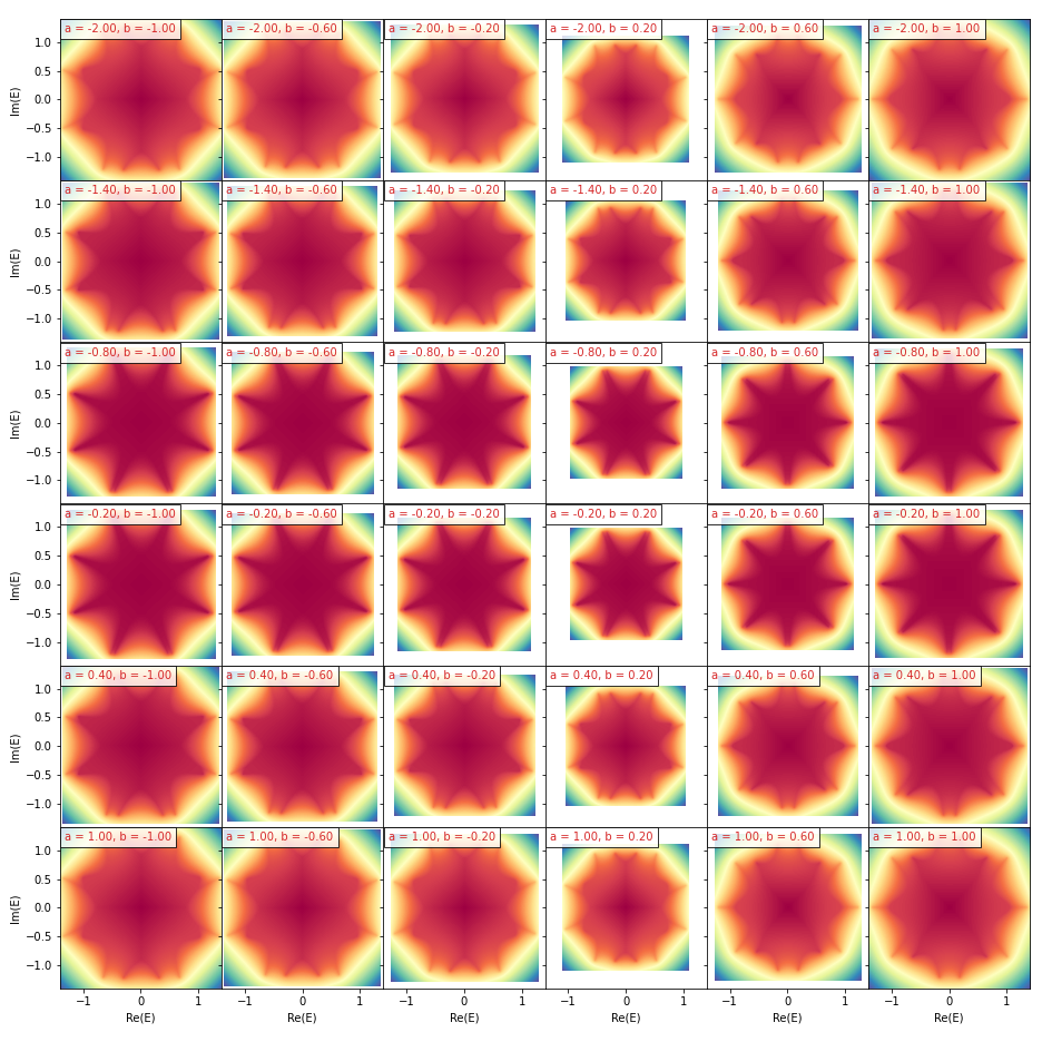
To get an array of spectral images or spectral graphs, we first prepare the values of the parameters {a,b}

a_array = np.linspace(-2, 1, 6)
b_array = np.linspace(-1, 1, 6)
a_grid, b_grid = np.meshgrid(a_array, b_array)
param_dict = {a: a_grid, b: b_grid}
print('a_grid shape:', a_grid.shape,
    '\nb_grid shape:', b_grid.shape)

>>>

a_grid shape: (6, 6)
b_grid shape: (6, 6)

Note that the value array of the parameters should have the same shape, which is also the shape of the output array of spectral images

phi_arr, dos_arr, binaried_dos_arr, spectral_square = \
    cp.spectral_images(param_dict=param_dict)
print('phi_arr shape:', phi_arr.shape,
    '\ndos_arr shape:', dos_arr.shape,
    '\nbinaried_dos_arr shape:', binaried_dos_arr.shape)

>>>

phi_arr shape: (6, 6, 1024, 1024) 
dos_arr shape: (6, 6, 1024, 1024) 
binaried_dos_arr shape: (6, 6, 1024, 1024)

from mpl_toolkits.axes_grid1 import ImageGrid

fig = plt.figure(figsize=(13, 13))
grid = ImageGrid(fig, 111, nrows_ncols=(6, 6), axes_pad=0, 
                 label_mode='L', share_all=True)

for ax, (i, j) in zip(grid, [(i, j) for i in range(6) for j in range(6)]):
    ax.imshow(phi_arr[i, j], extent=spectral_square[i, j], cmap='terrain')
    ax.set(xlabel='Re(E)', ylabel='Im(E)')
    ax.text(
        0.03, 0.97, f'a = {a_array[i]:.2f}, b = {b_array[j]:.2f}',
        ha='left', va='top', transform=ax.transAxes,
        fontsize=10, color='tab:red',
        bbox=dict(alpha=0.8, facecolor='white')
    )

plt.tight_layout()
plt.savefig('./assets/ChP_spectral_potential_grid.png', dpi=72)
plt.show()

---

An Array of Spectral Graphs

graph_flat, param_dict_flat = cp.spectral_graph(param_dict=param_dict)
print(graph_flat, '\n')
print(param_dict_flat)

[<networkx.classes.multigraph.MultiGraph object at 0x000001966DFCD190>, 
<networkx.classes.multigraph.MultiGraph object at 0x000001966DFCECF0>, 
...
<networkx.classes.multigraph.MultiGraph object at 0x000001966DFCE750>]

{a: 
array([-2. , -1.4, -0.8, -0.2,  0.4,  1. , -2. , -1.4, -0.8, -0.2,  0.4,
        1. , -2. , -1.4, -0.8, -0.2,  0.4,  1. , -2. , -1.4, -0.8, -0.2,
        0.4,  1. , -2. , -1.4, -0.8, -0.2,  0.4,  1. , -2. , -1.4, -0.8,
       -0.2,  0.4,  1. ]), 
b: 
array([-1. , -1. , -1. , -1. , -1. , -1. , -0.6, -0.6, -0.6, -0.6, -0.6,
       -0.6, -0.2, -0.2, -0.2, -0.2, -0.2, -0.2,  0.2,  0.2,  0.2,  0.2,
        0.2,  0.2,  0.6,  0.6,  0.6,  0.6,  0.6,  0.6,  1. ,  1. ,  1. ,
        1. ,  1. ,  1. ])}

Note

The spectral graph is a networkx.MultiGraph object, which cannot be directly returned as a multi-dimensional numpy array of MultiGraph, except for the case of 1D array. Instead, we return a flattened list of networkx.MultiGraph objects, and the accompanying param_dict_flat is the dictionary that contains the corresponding flattened parameter values.

Tip

It's recommended to pass the values of the parameters as vectors (1D arrays) instead of higher dimensional ND arrays to avoid the overhead of reshaping the output and the difficulty to retrieve / postprocess the spectral graphs.

Citation

If you find this work useful, please cite our paper:

@misc{yan2025hsg12mlargescalespatialmultigraph,
      title={HSG-12M: A Large-Scale Spatial Multigraph Dataset}, 
      author={Xianquan Yan and Hakan Akgün and Kenji Kawaguchi and N. Duane Loh and Ching Hua Lee},
      year={2025},
      eprint={2506.08618},
      archivePrefix={arXiv},
      primaryClass={cs.LG},
      url={https://arxiv.org/abs/2506.08618}, 
}