Study relationship between technical indicators and future Forex price
Technical analysis is a methodology for forecasting the direction of prices through past market data, primarily price and volume. Technical indicator normally apply to daily data. It would be interesting if we try to apply a minute data which much more variant and uncertainty.
Technical indicator has ability to reflect current status of price. Technical analysis uses indicators to help identify momentum, trends and volatility. Prediction power comes from analyser who interprete the signal.
We try to proof that technical indicator has enough power to predict the price in future. We will use very short time scale (1 minute period) to show how well this system handle inconsistent data.
In this study, we will use intelligent system to put indicator's signal together and forecast future price in form of Rate of Return.
Indicators which identify momentum, trends and volatility from price and volume.
-
RSI: identifies momentum, determines overbought and oversold conditions.
-
MACD: offers trend following and momentum.
-
ADX : measures trend strength without regard to trend direction.
-
BBand: are volatility bands placed above and below a moving average.
-
MFI: is an oscillator that uses both price and volume to measure buying and selling pressure.
We use USD - EUR exchange rate from Exness which is free and up to date.
Target for forecasting is 15 minutes ahead which traders can plan their strategy and rate of return is significantly different.
We decide to use regression model because this study aims to forecast rate of return in next 15 minutes. Regression analysis usually applies root-mean-square error (RMSE) as an error measurement. It shows deviations of the predictions from the true values. Less number is preferred.
Amount of transaction for test and train is 6000 between 2014.06.03 to 2014.06.10. We split 60/40 for training/testing following rule of thumb.
The model uses indicator values as its feature. We plot all features against each others too
Execute R code
# Prepare raw data
source("forex_study.R")`
data=get_caret_train_set("data/forex", "EURUSDe", "M1", 10000, n_period_forecast=15)
https://raw.githubusercontent.com/natapone/Project_ForexStudy/master/Images/plot_predictors.png
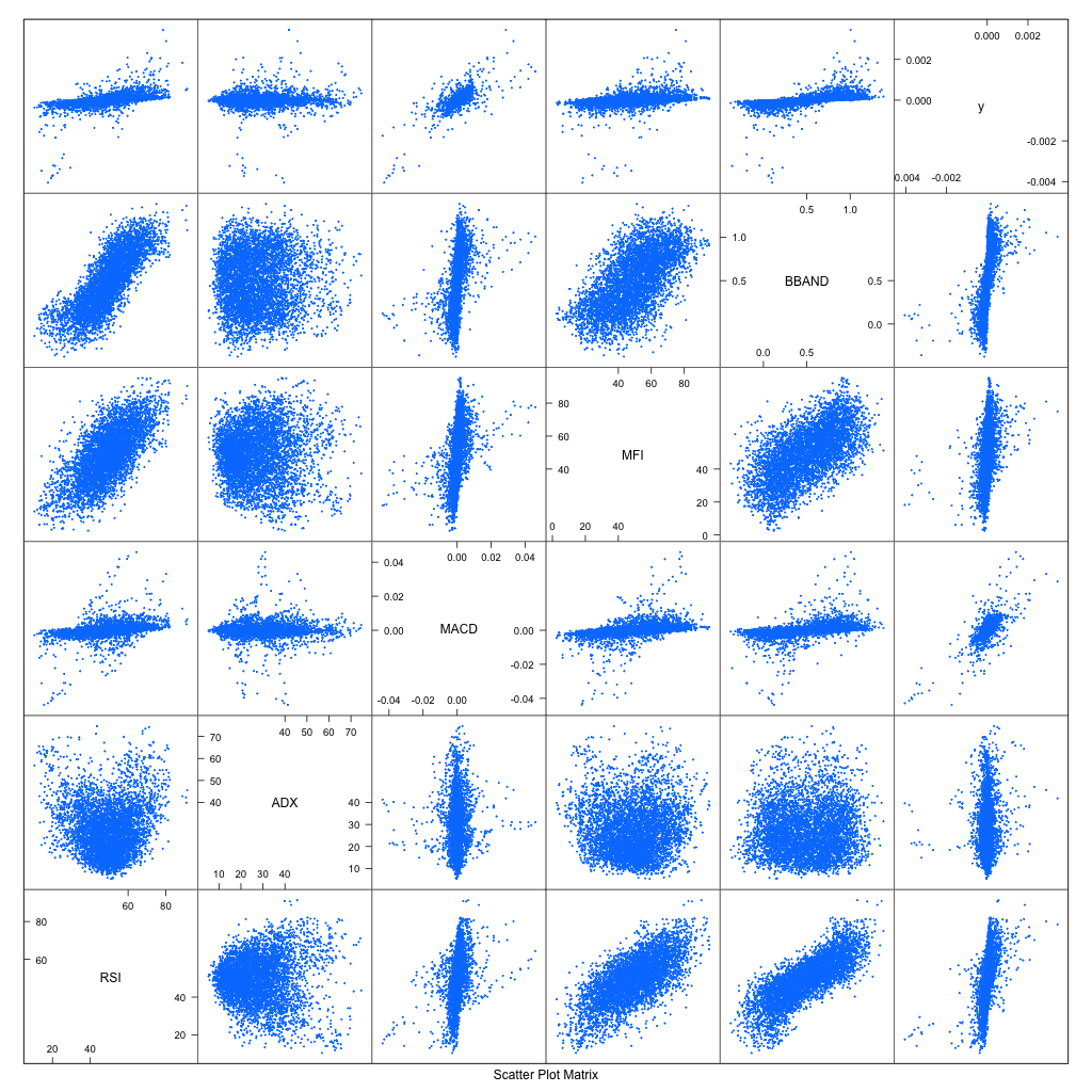
Focus on top rows, Rate of return (ROR) is plotted as y. We can roughly see that RSI, MFI and BBAND have similar relationship with ROR. MACD gathers around center , lower right and top left. ADX doesn't give any clue.
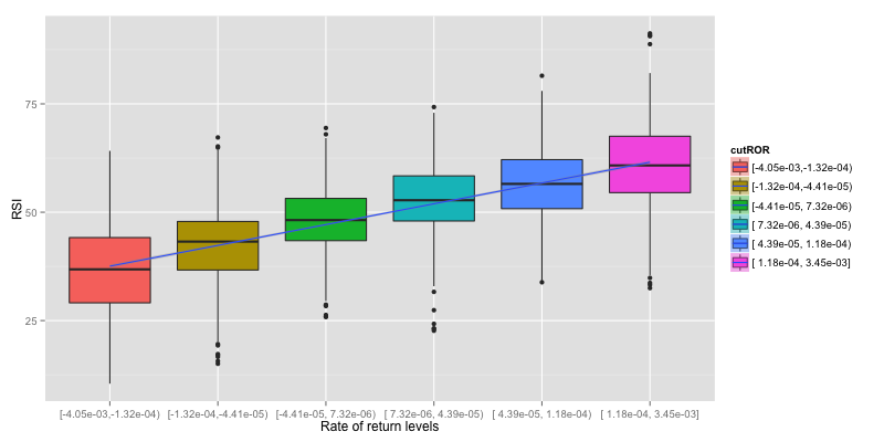
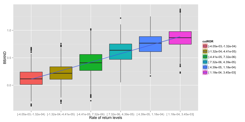
Plots are simplify as Boxplot to easily determine if there is a relationship between indicator and rate of return or not. To Simplify the plot, ROR is grouped in to 6 levels and linear regression line is drew on them to indicate how does indicator response to reate of return.
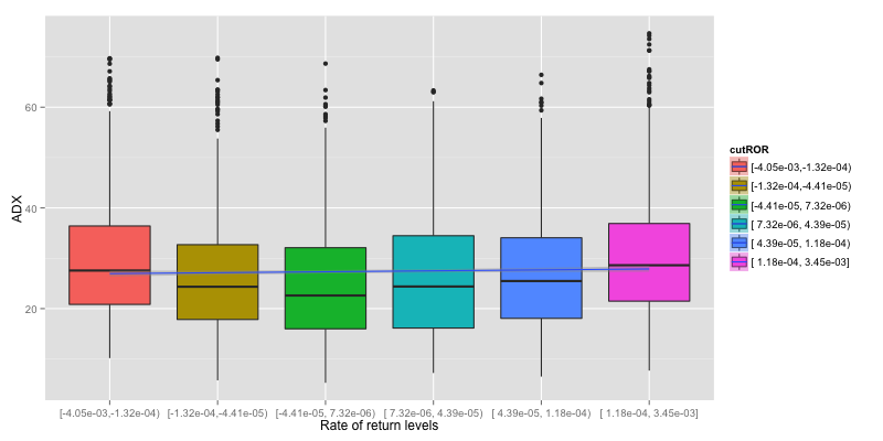
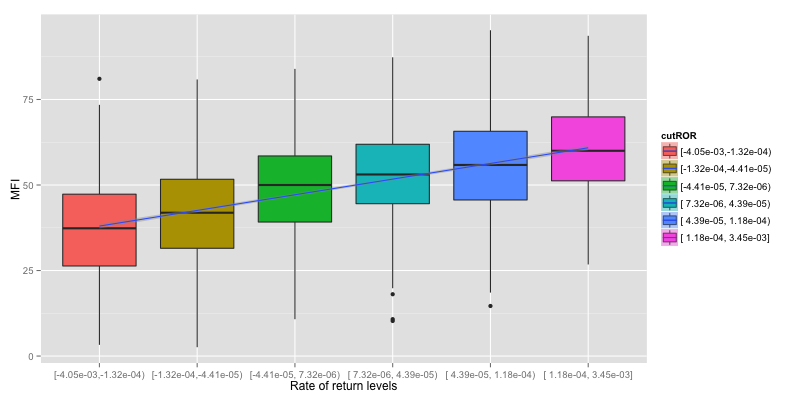
Now we can verify that ADX give no information about rate of return.
We choose generalized linear model (GLM) because it is flexible generalization for ordinary linear regression.
Execute R code
forex_train_model(data)
Result of GLM training Measure GLM RMSE
Generalized Linear Model

3552 samples
   5 predictors

No pre-processing
Resampling: Bootstrapped (25 reps)

Summary of sample sizes: 3552, 3552, 3552, 3552, 3552, 3552, ...

Resampling results

  RMSE      Rsquared  RMSE SD   Rsquared SD
  0.000222  0.708     1.38e-05  0.0315
RMSE number is good for comparing model. but it doesn't give any picture of how well it predict. We interprete the result by;
-
If rate of return > 0, count as PROFIT (1)
-
If rate of return <= 0, count as LOSE (-1)
And plot confusion matrix to visualization of the performance of an algorithm.
Measure GLM accuracy
Confusion Matrix and Statistics

          Reference
Prediction   -1    1
        -1 1015  200
        1   230  920

               Accuracy : 0.8182
                 95% CI : (0.802, 0.8335)
    No Information Rate : 0.5264
    P-Value [Acc > NIR] : <2e-16

                  Kappa : 0.6358
 Mcnemar's Test P-Value : 0.162

            Sensitivity : 0.8153
            Specificity : 0.8214
         Pos Pred Value : 0.8354
         Neg Pred Value : 0.8000
             Prevalence : 0.5264
         Detection Rate : 0.4292
   Detection Prevalence : 0.5137
      Balanced Accuracy : 0.8183

       'Positive' Class : -1
GLM model accuracy from estimation above is 81.8% which is quite high. But there is a room for improvement
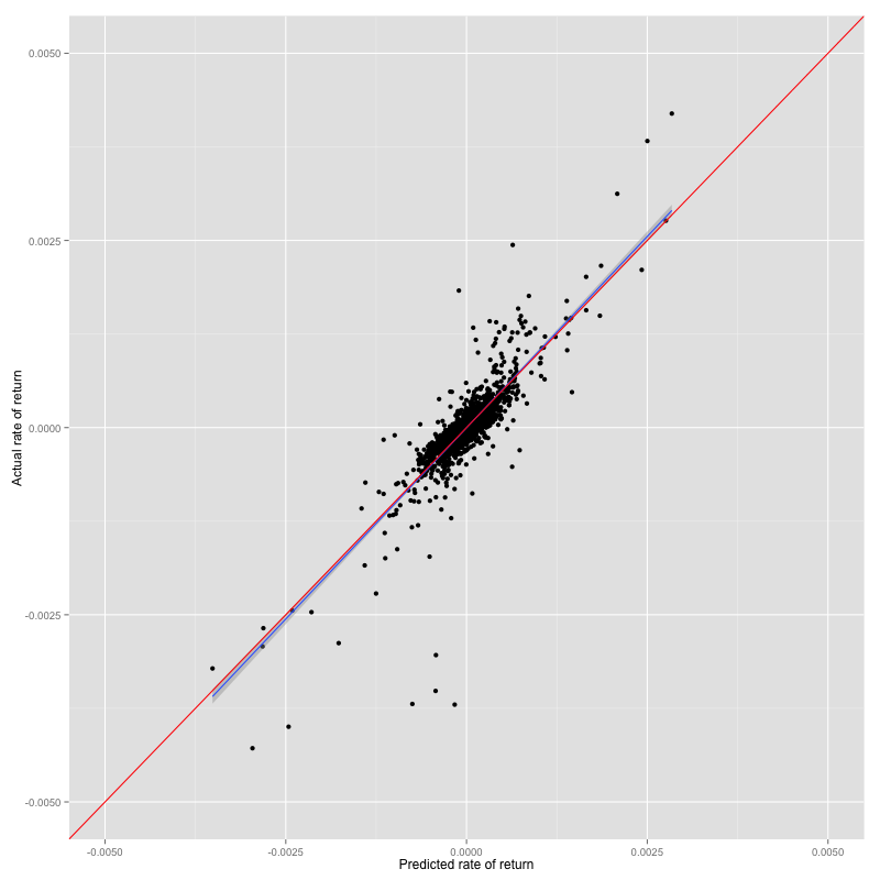
We plot prediction result against actual rate of return to show how effective the algorithm is. The diagonal line(red) is ideal condition, dot closer to the line is preferred. Linear regression line(blue) of the plot shows relationship between prediction and actual. Blue line should be on red line in ideal case.
Prediction result vs test set of GLM
We analyse in further detail to optimize the model.
Simplify plots show that ADX give no relationship to rate od return. RSI, MFI and BBAND return similar pattern. We can remove some indicators to keep model as simple as possible. We rebuild model again with RSI and MACD then look at the result.
Execute R code
d1 = model_improve_1(data)
Measure RMSE of GLM improvement
Generalized Linear Model

3552 samples
   2 predictors

No pre-processing
Resampling: Bootstrapped (25 reps)

Summary of sample sizes: 3552, 3552, 3552, 3552, 3552, 3552, ...

Resampling results

  RMSE      Rsquared  RMSE SD   Rsquared SD
  0.000224  0.7       1.41e-05  0.0312
Measure accuracy
Confusion Matrix and Statistics

          Reference
Prediction   -1    1
        -1 1021  156
        1   224  964

               Accuracy : 0.8393
                 95% CI : (0.8239, 0.8539)
    No Information Rate : 0.5264
    P-Value [Acc > NIR] : < 2.2e-16

                  Kappa : 0.6787
 Mcnemar's Test P-Value : 0.0005881

            Sensitivity : 0.8201
            Specificity : 0.8607
         Pos Pred Value : 0.8675
         Neg Pred Value : 0.8114
             Prevalence : 0.5264
         Detection Rate : 0.4317
   Detection Prevalence : 0.4977
      Balanced Accuracy : 0.8404

       'Positive' Class : -1
Prediction result vs test set of GLM improvment
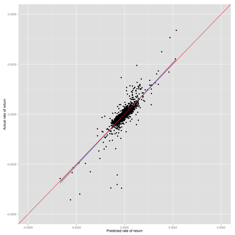
The result shows that RMSE is slightly increase but accuracy is about 2% increase even we remove three indicators. We can use only RSI and MACD to build the model without decrease its prediction power.
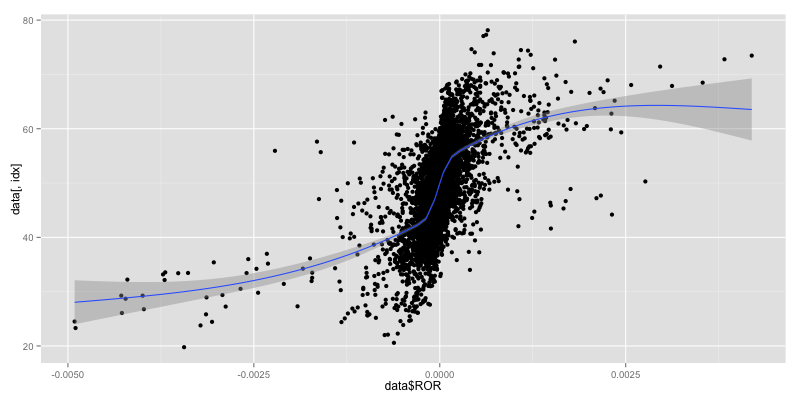
Take a look at RSI vs ROR closely, we can see that the relationship is not linear. We plot regression line again with non-linear smoothing technique.
Plot non-linear RSI
We use svmPoly or Support Vector Machines with Polynomial Kernel which is non linear model.
Execute R code
model_improve_2(d1)
Measure RMSE of svmPoly
Support Vector Machines with Polynomial Kernel

3552 samples
   2 predictors

No pre-processing
Resampling: Bootstrapped (25 reps)

Summary of sample sizes: 3552, 3552, 3552, 3552, 3552, 3552, ...

Resampling results across tuning parameters:

  degree  scale  C     RMSE      Rsquared  RMSE SD   Rsquared SD
  1       0.001  0.25  0.000297  0.693     2.13e-05  0.0293
  1       0.001  0.5   0.000265  0.701     1.91e-05  0.0319
  1       0.001  1     0.000247  0.699     1.78e-05  0.034
  1       0.01   0.25  0.000237  0.695     1.64e-05  0.0356
  1       0.01   0.5   0.000234  0.693     1.58e-05  0.0361
  1       0.01   1     0.000233  0.692     1.57e-05  0.0364
  1       0.1    0.25  0.000232  0.691     1.56e-05  0.0367
  1       0.1    0.5   0.000232  0.691     1.57e-05  0.0368
  1       0.1    1     0.000232  0.69      1.56e-05  0.0368
  2       0.001  0.25  0.000265  0.701     1.92e-05  0.0319
  2       0.001  0.5   0.000246  0.7       1.78e-05  0.034
  2       0.001  1     0.000238  0.697     1.68e-05  0.0355
  2       0.01   0.25  0.000232  0.697     1.65e-05  0.0377
  2       0.01   0.5   0.000231  0.695     1.62e-05  0.0382
  2       0.01   1     0.00023   0.693     1.61e-05  0.0388
  2       0.1    0.25  0.000231  0.69      1.65e-05  0.0397
  2       0.1    0.5   0.000231  0.69      1.65e-05  0.0397
  2       0.1    1     0.000231  0.69      1.64e-05  0.0396
  3       0.001  0.25  0.000253  0.701     1.82e-05  0.0332
  3       0.001  0.5   0.00024   0.699     1.72e-05  0.0349
  3       0.001  1     0.000235  0.696     1.64e-05  0.036
  3       0.01   0.25  0.000226  0.703     1.6e-05   0.0381
  3       0.01   0.5   0.000225  0.705     1.58e-05  0.0377
  3       0.01   1     0.000222  0.709     1.54e-05  0.0374
  3       0.1    0.25  0.000214  0.728     2.05e-05  0.0453
  3       0.1    0.5   0.000215  0.727     2.1e-05   0.0469
  3       0.1    1     0.000215  0.727     2.1e-05   0.0465

RMSE was used to select the optimal model using  the smallest value.
The final values used for the model were degree = 3, scale = 0.1 and C = 0.25.

The optimal RMSE = 0.000214
Measure accuracy of svmPoly
Confusion Matrix and Statistics

          Reference
Prediction   -1    1
        -1 1036  168
        1   209  952

               Accuracy : 0.8406
                 95% CI : (0.8252, 0.8551)
    No Information Rate : 0.5264
    P-Value [Acc > NIR] : < 2e-16

                  Kappa : 0.6809
 Mcnemar's Test P-Value : 0.03939

            Sensitivity : 0.8321
            Specificity : 0.8500
         Pos Pred Value : 0.8605
         Neg Pred Value : 0.8200
             Prevalence : 0.5264
         Detection Rate : 0.4381
   Detection Prevalence : 0.5091
      Balanced Accuracy : 0.8411

       'Positive' Class : -1
Prediction result vs test set of svmPoly
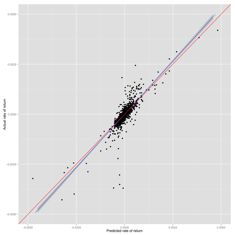
Changing model to non-linear improves 2% accuracy but slope of prediction result and actual is slightly worse.
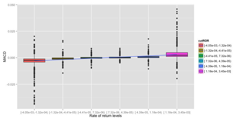
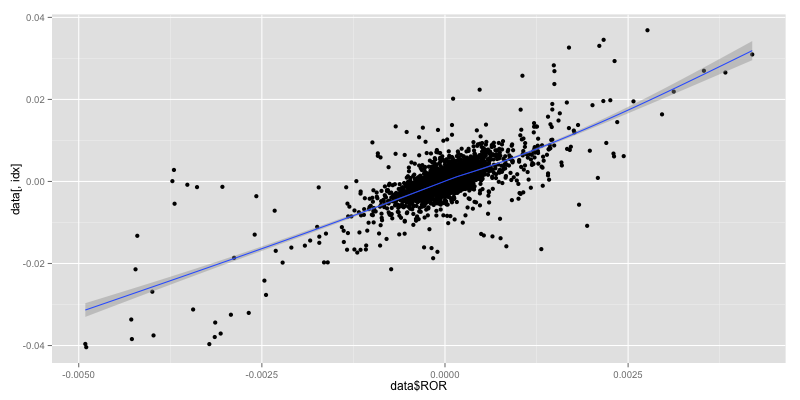
There is an improvement point from MACD scatter plot. MACD vs ROR seem to group into small cluster with linear relationship.
Scatter plot MACD
We choose Regression Trees Model which is Prediction trees that return regression result. It use the tree to represent the recursive partition.
Execute R code
model_improve_2(d1)
Measure RMSE of M5
Model Tree

3552 samples
   2 predictors

No pre-processing
Resampling: Bootstrapped (25 reps)

Summary of sample sizes: 3552, 3552, 3552, 3552, 3552, 3552, ...

Resampling results across tuning parameters:

  pruned  smoothed  rules  RMSE      Rsquared  RMSE SD   Rsquared SD
  Yes     Yes       Yes    0.000209  0.741     1.66e-05  0.0317
  Yes     Yes       No     0.000206  0.748     1.55e-05  0.0335
  Yes     No        Yes    0.00021   0.739     1.67e-05  0.0319
  Yes     No        No     0.00023   0.691     2.93e-05  0.0567
  No      Yes       Yes    0.000223  0.711     1.53e-05  0.0292
  No      Yes       No     0.000205  0.748     1.5e-05   0.0309
  No      No        Yes    0.000272  0.592     2.23e-05  0.0584
  No      No        No     0.000266  0.612     1.34e-05  0.0405

RMSE was used to select the optimal model using  the smallest value.
The final values used for the model were pruned = No, smoothed = Yes and rules = No.

The optimal RMSE = 0.000205
Measure accuracy of M5
Confusion Matrix and Statistics

          Reference
Prediction   -1    1
        -1 1020  167
        1   225  953

               Accuracy : 0.8342
                 95% CI : (0.8186, 0.849)
    No Information Rate : 0.5264
    P-Value [Acc > NIR] : < 2e-16

                  Kappa : 0.6684
 Mcnemar's Test P-Value : 0.00399

            Sensitivity : 0.8193
            Specificity : 0.8509
         Pos Pred Value : 0.8593
         Neg Pred Value : 0.8090
             Prevalence : 0.5264
         Detection Rate : 0.4313
   Detection Prevalence : 0.5019
      Balanced Accuracy : 0.8351

       'Positive' Class : -1
Prediction result vs test set of M5
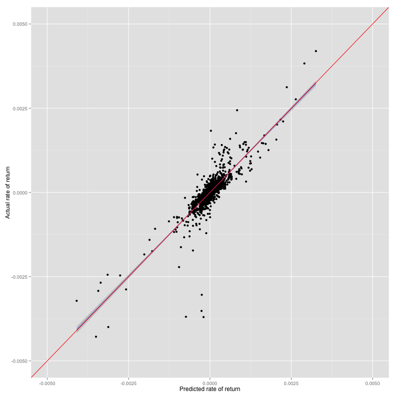
RMSE is improve but accuracy is slightly decreased. The most interesting result is slope of prediction - actual relationship is on the ideal line.
There are three dimensions that we use to determine the model performance which are RMSE, accuracy and relationship slope. Only way to proof is through the real trade. Next phase we'll construct automate trading bot with these algorithms to demonstrate how they response to the real situation.